Use of Vehicle Dynamic Model in robust mapping
January 2023
By Kenneth Joseph Paul, a PhD student at EPFL.
The objective of the GAMMS H2020 project is to develop autonomous mapping systems capable of producing high-definition maps. A major challenge in urban mapping scenarios is the estimation of the position of the vehicle during conditions when GNSS signals are not available. The role of EPFL in this project is to tackle this challenge by bringing in an innovative method that mathematically constrains the estimation of vehicle motion. These constraints are encapsulated using a synthetic sensor based on the Vehicle Dynamic Model (VDM).
In the field of autonomous robot navigation, estimation of position and orientation within a frame of reference is essential. This information is estimated using the measurements from different sensors mounted on the robot – for instance, GNSS and Inertial Measurement Unit (IMU). However, sensor measurements are not perfect due to electromechanical disturbance. Hence, relying only on a single type of sensor can lead to suboptimal estimates of position and orientation. This issue is solved by a process known as sensor fusion.
Conventional sensor fusion
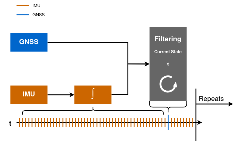
Sensor fusion is the process by which measurements from different types of sensors are combined to determine the best possible estimate for the position and orientation. The conventional approach is based on i) kinematic modelling and ii) recursive estimation of state-space variables. As shown in the above schematic, the GNSS and IMU measures are recursively fused together to obtain the best estimate for the position and orientation. Kinematic modelling depends only on the IMU measurements – which are always available. This makes the whole process independent of the vehicle. In other words, sensor fusion can be used on any vehicle, be it aerial or terrestrial, to estimate its position and orientation. An advantage of this method is the recursivity in estimation by means of Bayesian Filtering (for instance the Kalman filter). This allows keeping in memory only the recent navigation state (position, velocity, orientation) together with its confidence, the reason for which is computationally efficient and well suited for real-time operation.
Figure 1 - Kalman Filtering
The GNSS and IMU measurements are recursively fused. The time axis at the bottom shows sensor measurements arriving at different time instances. Only the latest state is stored in the memory
GAMMS sensor fusion
Both previously mentioned advantages in conventional sensor fusion can be questioned when there is a need to maximize the quality of trajectory estimation as in the scenarios where GNSS signal reception is intermittent and where the estimate can be delayed in time, which is the case of mapping. In such situations, it may be better to consider dynamic modelling and consider all observations over all epochs together. This is the GAMMS approach.
Trajectory estimation can benefit from optical sensor measurement, but this requires the need to access past states to integrate them into the sensor fusion pipeline. Such constraints on measurements are spatial. This is difficult to achieve within the conventional sensor fusion together with raw IMU data that are constraining the trajectory temporally. Also, the conventional sensor fusion technique allows only one type of modelling (e.g., kinematic or dynamic). In order to overcome these challenges, GAMMS adopts a sensor fusion technique known as Dynamic Network (DN) to which EPFL adds the vehicle dynamic model.
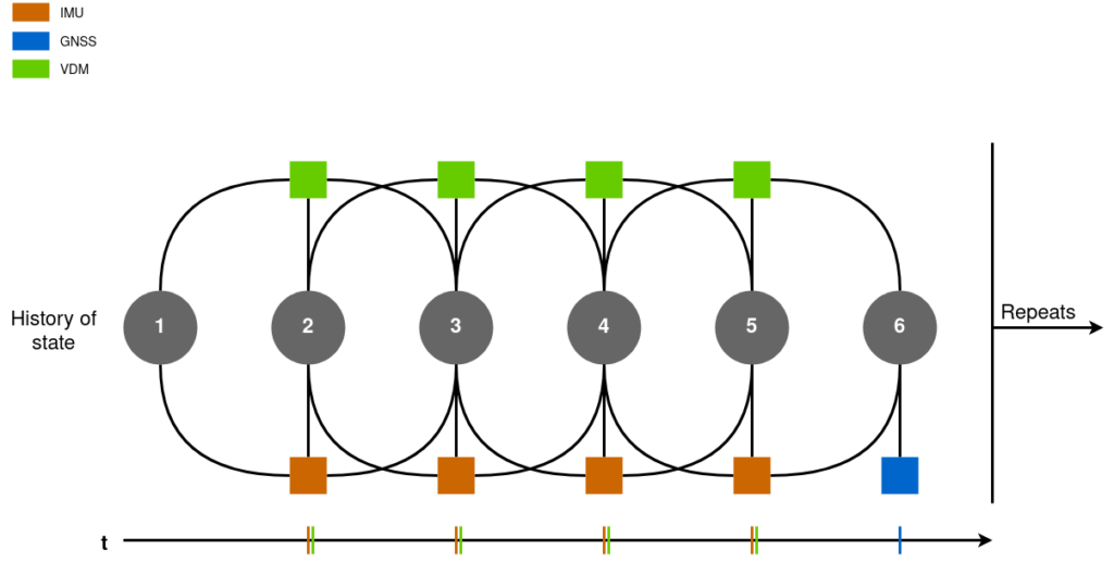
The figure below is a simplified schematic of a DN. The circles in the grey represent the states of the vehicle for that specific time instance. The measurements in the network constrain these states using equations known as observation models. The number of states constrained by a measurement depends on the order of measurement type (e.g. a second-order measurement like linear acceleration constraints 3 states in time). These constraints can be both spatial and temporal. The advantages of using spatial constraints such as lidar measurements with DN have been discussed in detail in the work [1]. All observations from navigation and optical sensors are compensated together at once, which is the optimal approach to mitigate drifts during GNSS signal absence. At the same time, the motion can be further constrained via a mathematical model, as proposed by EPFL.
Figure 2 - Dynamic Network
The circles in the grey represent the states of the vehicle for that specific time instance. The squares represent the different sensor measurements. Measurements and states are constrained by equations known as the observation model. The time axis at the bottom shows sensor measurements arriving at different time instances
Vehicle Dynamic Model
Locomotion in robots (like automated cars) is achieved with the help of actuators. When a control command is issued to the actuator, it applies a force and torque on the body, which in turn produces a linear and angular acceleration according to the laws of motion. This relationship between the control inputs and acceleration can easily be obtained for various platforms. Therefore, without the need to add additional sensors to the platform, a new type of measurement is available for sensor fusion. As shown in [2] for a fixed-wing drone, using VDM measurements when GNSS is not available reduces the uncertainty in the position and orientation significantly. The simplified VDM model for a car is provided in the figure below.
Figure 3 - Vehicle Dynamic Model for a car
The wheels' steering angles and rotation speed are inputs to the VDM mode. The VDM parameters are different coefficients in the equations such as the car's mass, wheel's radius, inertia matrix, etc.
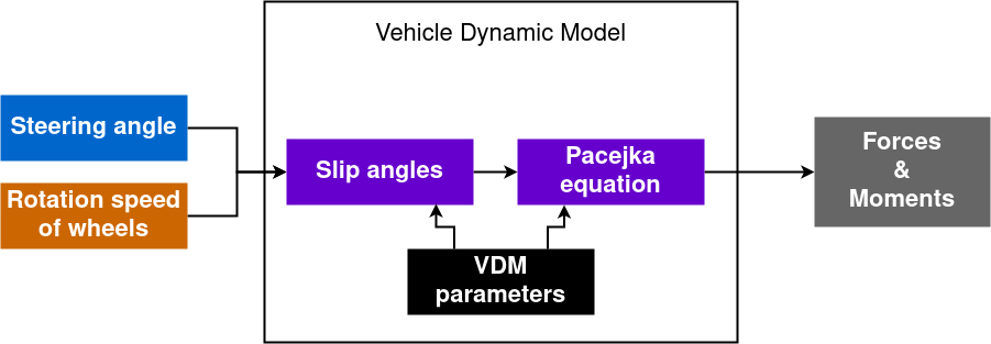
Once the angles of slip are calculated, forces acting on tires can be evaluated using the Pacejka equation [3]
F = Fz * D * sin( C * arctan( B * slip – E * ( B * slip – arctan( B * slip ))))
Fz is the vertical force at the tire and the parameters B, C, D, E depend on road conditions. The addition of VDM measurements allows the autonomous vehicle to improve the quality of its estimated position in areas with poor or no GNSS signals. This measurement can be principally used either in conventional or GAMMS sensor fusion, but it is intended for the latter to improve mapping quality.
References
- A. Brun, D. A. Cucci, and J. Skaloud, “Lidar point–to–point correspondences for rigorous registration of kinematic scanning in dynamic networks,” ISPRS Journal of Photogrammetry and Remote Sensing, vol. 189, pp. 185–200, 2022-07, doi: 10.1016/J.ISPRSJPRS.2022.04.027.
- M. Khaghani and J. Skaloud, “Assessment of VDM-based autonomous navigation of a UAV under operational conditions,” Robotics and Autonomous Systems, vol. 106, pp. 152–164, 2018-08, doi: 10.1016/J.ROBOT.2018.05.007.
- H. Pacejka, Tire and vehicle dynamics. Elsevier, 2005.